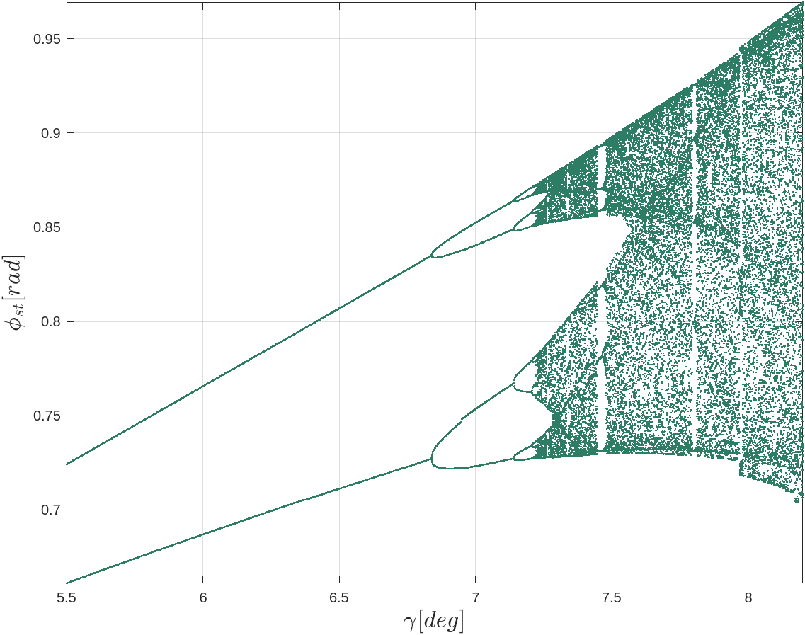
(a)
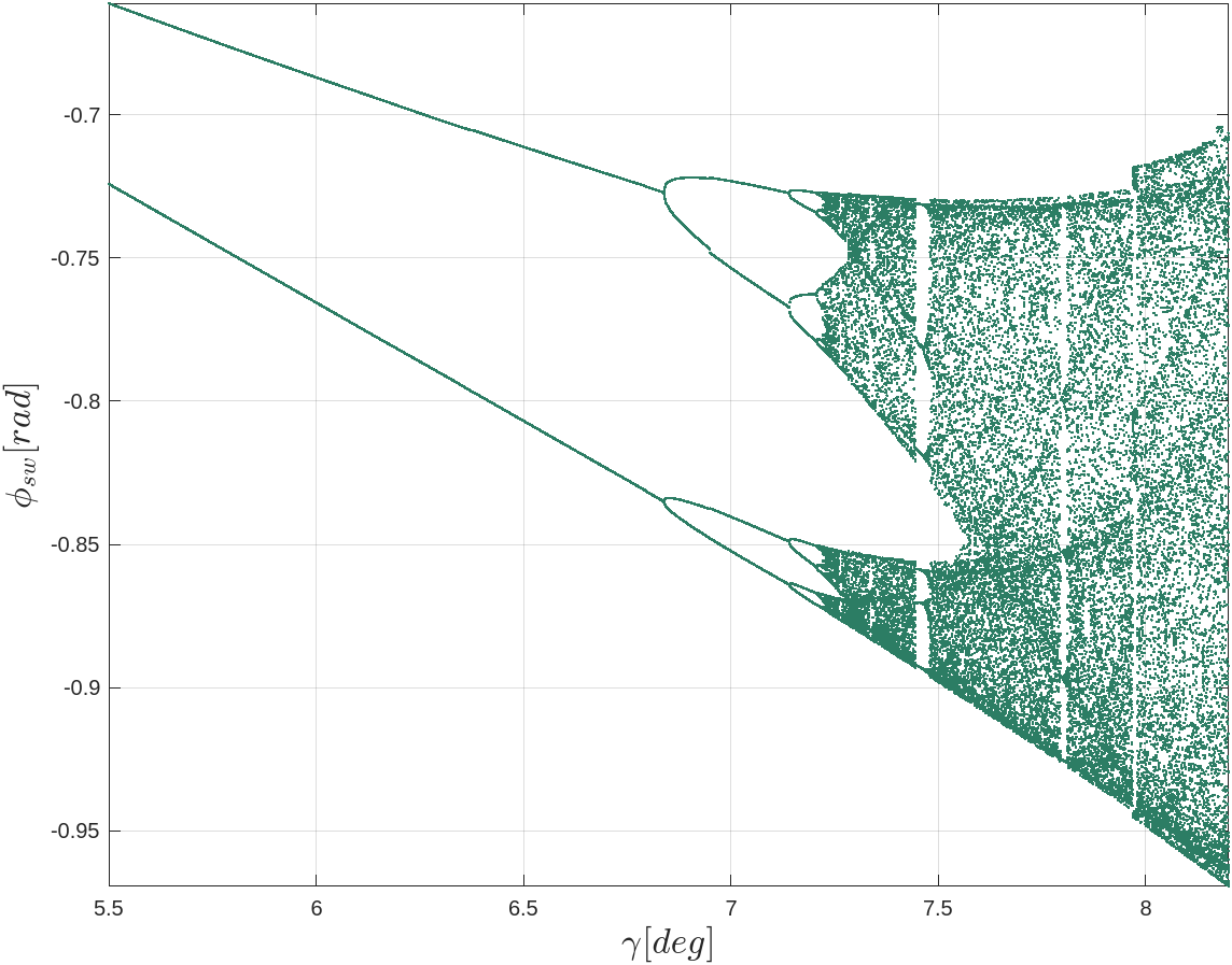
(b)
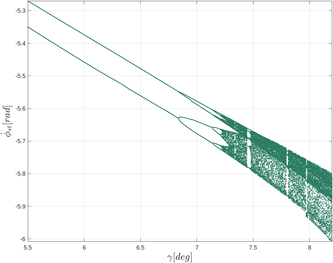
(c)
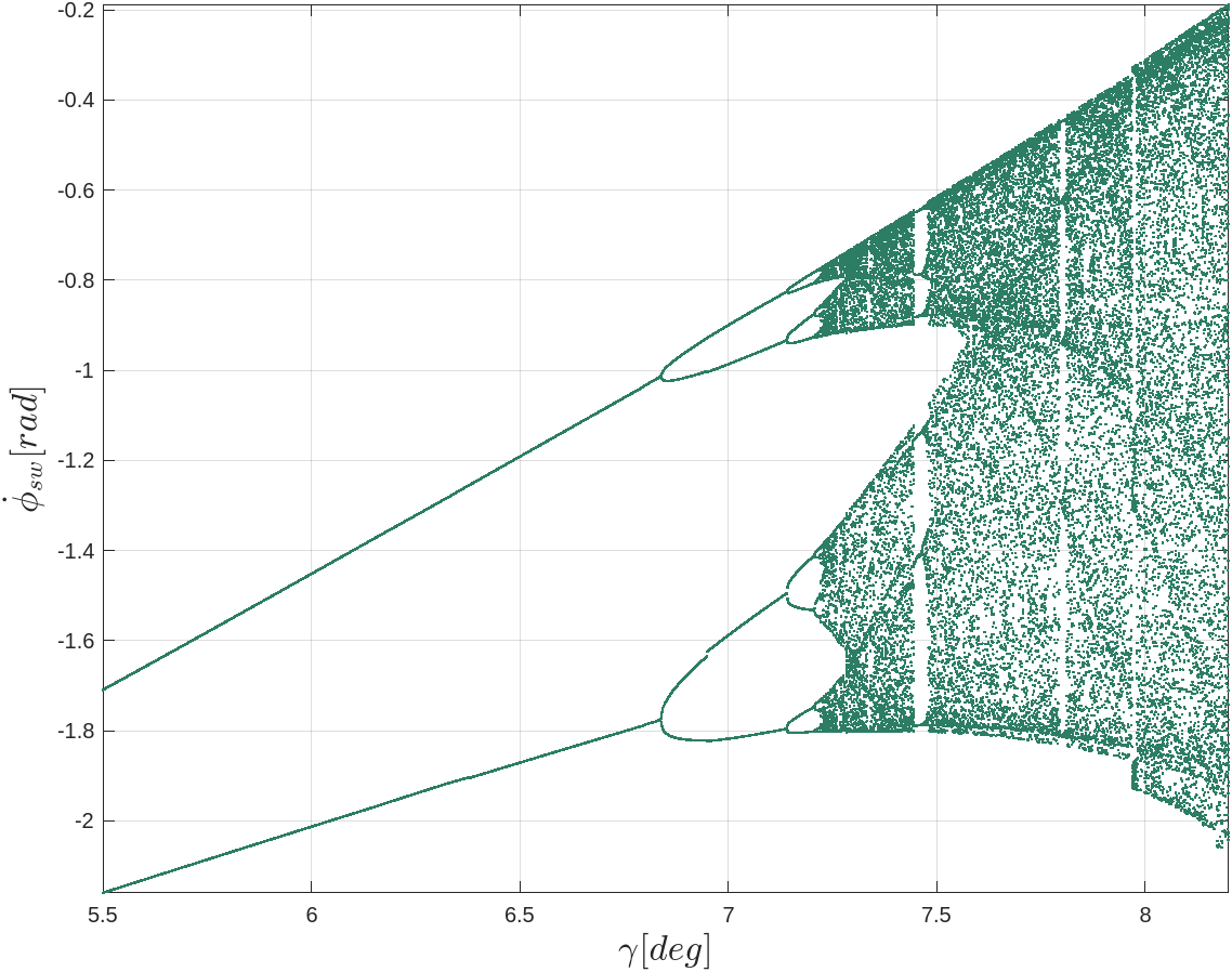
(d)
Bifurcation of system states: (a) $\phi_{st}$, (b) $\phi_{sw}$, (c) $\dot{\phi}_{st}$, (d) $\dot{\phi}_{sw}$
Jun 13, 2020
Compass-gait bipedal walkers have been studied extensively as a fundamental model in robotics and locomotion. Their kinematics are motivated by the pendular efficiencies of human walking.
For this project, I modeled a compass-gait walker as a passive system. Its movement, thus, relies solely on gravity and the resulting pendular motion of its legs.
The focus of this project is to model the equations of motion, derived using a combination of Newton-Euler and Lagrangian mechanics (TMT-method, presented by Vallery and Schwab[1]). Additionally, after the walker is modeled, its interaction with the incline surface can be observed. From these simulations, we are able to observe limit cycles, bifurcation, and eventually, chaos!
The system is modeled and simulated entirely within MATLAB computing environment.
The walker consists of two identical rigid legs connected at a frictionless hip joint. Each leg has a curved foot (radius R) that rolls on a slope inclined at angle $\gamma$. The leg length L is measured from the center of the foot arc to the hip. The CoM of each leg is located at a position (B, C) relative to the hip, where B is the horizontal offset and C is the vertical offset (positive downward from hip toward foot).
The sketch below shows the configuration during the swing phase, with the stance leg rolling on the ground and the swing leg freely rotating about the hip. The stance leg and swing leg are denoted by subscripts \(st\) and \(sw\), respectively.
Compass gait walker with curved feet (radius R) and offset CoM. Stance leg (left) rolls on slope; swing leg (right) rotates freely about hip
| Parameter | Symbol | Description |
|---|---|---|
| Leg length | $L$ | Distance from foot arc center to hip joint |
| Foot radius | $R$ | Radius of circular arc foot |
| CoM offset, horizontal | $B$ | Horizontal distance of CoM from hip |
| CoM offset, vertical | $C$ | Vertical distance of CoM from hip (towards foot) |
| Leg mass | $m$ | Point mass at each leg CoM |
| Leg moment of inertia | $I$ | Rotational inertia at each leg about its CoM |
| Slope angle | $\gamma$ | Downhill inclination of the walking surface |
| Gravitational acceleration | $g$ | 9.81 $\text{m}/\text{s}^2$ |
| Roll friction | $r_f$ | Rolling resistance at stance foot |
| Hip friction | $h_f$ | Viscous friction at hip joint |
The system has two degrees of freedom, described by the generalized coordinate vector: $$ q = \begin{bmatrix} \phi_{st} \\ \phi_{sw} \\ \end{bmatrix} $$
where $\phi_{st}$ is the counter-clockwise angle of the stance leg and $\phi_{stw}$ is the counter-clockwise angle of the swing leg, both measured from normal to the incline slope. Thus, the full state vector integrated by the ODE solver is:
$$ s=\begin{bmatrix} \phi_{st} & \phi_{sw} & \dot{\phi}_{st} & \dot{\phi}_{sw} \end{bmatrix}^\top $$The TMT method is a systematic way to derive Equations of Motion (EOM) for constrained multi-body systems. The name comes from the matrix product $T^\top MT$ that defines the reduced mass matrix. It avoids explicit computation of constraint forces by projecting Newton's law from the full physical space into the generalized-coordinate space via the kinematic Jacobian $T$.
The method proceeds in four steps:
The full physical descriptor state \(x \in \mathbb{R}^6\) stacks the planar positions and angles of both leg CoMs:
$$
x=\begin{bmatrix}
x_{st} & y_{st} & \phi_{st} & x_{sw} & y_{sw} & \phi_{sw}
\end{bmatrix}^\top
$$
The stance leg hip position, accounting for rolling contact of the curved foot on the slope, is: $$ p_h=\begin{bmatrix} -R\phi_{st} - (L-R)\sin(\phi_{st}) \\ R + (L-R)\cos(\phi_{st}) \end{bmatrix} $$
Note that the $-R\phi_{st}$ term is the arc-length rollout along the slope surface. The CoM of each leg is then obtained by rotating the offset (B, -C) from the hip by the leg’s angle: $$ p_{CoM}= p_{h} + \text{R}(\phi)\cdot \begin{bmatrix} B \\ -C \end{bmatrix} $$
where $\text{R}(\phi) = \begin{bmatrix}\cos\phi & -\sin\phi \\ \sin\phi & \cos\phi\end{bmatrix}$ is the 2D rotation matrix.
The Jacobian $T = \frac{\partial x}{\partial q} \in \mathbb{R}^{6\times2}$ maps generalized velocities to physical velocities: $$ \dot{x} = T\cdot\dot{q} $$
We can compute it symbolically using MATLAB’s jacobian() function. The resulting matrix can then be numerically evaluated at each time step to simulate physical motion of the walker.
The centripetal and Coriolis accelerations arise from the time derivative of $T\cdot\dot{q}$. They are computed as $$ D = \frac{\partial T\cdot\dot{q}}{\partial q} \cdot \dot{q} $$
In MATLAB, the above two can computed like so:
T = jacobian(x,q);
D = jacobian(T*qd,q)*qd;Equations of motion with constraint forces: $$ M\ddot{x} = f_{applied} + f_{constraint} $$
by principle of virtual work, constraint forces do no work along admissible motions: $$ f_{constraint} \in \text{null}(T) \quad \Longleftrightarrow \quad T^\top f_{constraint} = 0 $$
pre-multiply Newton's law by $T^\top$: $$ T^\top M\ddot{x} = T^\top f - T^\top MD \; + \; \underbrace{T^\top f_{constraint}}_{=0} $$ Substituting the kinematic identity $\ddot{x} = T\ddot{q} + D$ gives the reduced system: $$ \underbrace{(T^\top M T)}_{M_r} \ddot{q} = T^\top f - T^\top MD $$
where the physical mass matrix is block-diagonal is $$ M = \text{diag}(m, m, I, m, m, I) $$
and the gravitational force vector on a slope of angle $\gamma$ is $$ f = M\cdot g \cdot \begin{bmatrix} \sin\gamma & -\cos\gamma & 0 & \sin\gamma & -\cos\gamma & 0 \end{bmatrix}^\top $$
Defining the reduced 2×2 mass matrix $M_r \equiv T^\top M T$, the governing equation of motion is: $$ \boxed{M_r(\phi_{st},\phi_{sw})\cdot\ddot{q} = T^\top f - T^\top M D} $$ This is a 2×2 linear system solved at each time step for $\ddot{q} = \begin{bmatrix}\ddot{\phi_{st}}&\ddot{\phi_{st}}\end{bmatrix}^\top$
$M_r = T^\top M T$ is a symmetric 2x2 matrix. Its (2,2) entry has a notable simplification: the swing leg’s effective inertia about the hip reduces to $m(B^2 + C^2) + I$, which is constant and independent of the leg angle $\phi_{sw}$. This occurs because rotating T_{4:6,2} by any angle preserves its norm. The (1,1) entry and off-diagonal terms remain configuration-dependent through φ_st and φ_sw.
Optional rolling friction ($r_f$) at the stance foot and viscous hip friction ($h_f$) are included as generalized forces added to the right-hand side:
$$ \begin{align*} \text{fric} &= \begin{bmatrix} -r_f\dot{\phi}_{st} \\ 0 \end{bmatrix} + \begin{bmatrix} -h_f\dot{p}_h \\ h_f\dot{p}_h \end{bmatrix}\qquad, \; \dot{p}_h = \dot{phi}_{st} - \dot{phi}_{sw}\\\\ &=\begin{bmatrix} -r_f \dot{\phi}_{st} - h_f(\dot{\phi}_{st} - \dot{\phi}_{sw}) \\ h_f(\dot{\phi}_{st}-\dot{\phi}_{sw}) \end{bmatrix} \end{align*} $$For this project, friction has been set to zero for both $h_f$ and $r_f$.
Contact and collision in the system is characterized by non-slip and no-bounce contact. Under such definition, translational momentum at the point of contact is not conserved. This simplification is reasonable for most low road grade simulations, where impact is relatively low. In this project, the system is necessarily operated at low road grades, because beyond a certain angle \(\gamma\), it is not possible to keep the walker from falling over. Furthermore, it allows us to reduce the number of states to simulate, as the position and translational velocities of the legs become coupled with the angle and angular velocities of the legs.
The post-impact dynamics, in terms of generalized velocities $\dot{q}^+$, is thus $$ T_{sw}^\top M T_{sw}\cdot \dot{q}^+ = T_{sw}^\top M \cdot \dot{x}^- $$
In order to observe bifurcation of the system, the walker should be maintained such that it does not fall over. If the robot were to fall over, its corresponding states likely do not belong to a limit-cycle we are interested in.
To aid in observing its limit cycles, the walker begins its simulated walk at an inital state close to one of its attractors. Doing so helps to
It typically takes some number of steps before the system begins to settle towards its attractors; and that to observe bifurcation, many more additional steps are required to observe their periodic orbits. According to Strogatz, observing bifurcation requires on the order of a few hundred cycles (~300) per parameter value[2]. Consequently, producing a bifurcation diagram over a range of values for a system variable (in this case, \(\gamma\)) quickly becomes computationally intensive, as each cluster of points on the diagram requires hundreds of simulation steps.
For the following orbit diagrams, I simulated the system across approximately 10,000 increments of \(\gamma\). At each value of \(\gamma\), the walker completed 600 steps, and the system states at the moment of impact were recorded and plotted against the corresponding road grade. The resulting diagrams clearly demonstrate that the system states exhibit bifurcation and chaotic behavior.
An animation of the walker, created by plotting the system states over time in MATLAB, provides a visual confirmation of the model's behavior. This sanity check helps verify that the equations of motion and impact model were implemented correctly.