Introduction

In this project, I use reinforcement learning techniques to train a computer agent to play the game of Tetris. The goal of an intelleigent agent in this game is straightforward: to clear as many rows as possible.

At first glance, one might try to train and optimize the agent such that it clears as many rows as possible at each stage. However, through experiments, it quickly becomes clear that such a direct or "greedy" policy does not yield a very intelligent agent.

Tetris is an NP-complete problem, which means finding a perfect sequence of moves is computationally intractable. Furthermore, since the agent has no knowledge of future pieces, its performance can only be truly assessed after a game is complete. A simple "greedy" policy that only tries to clear rows at each step performs poorly as it forgoes any board optimization for future stages. Luckily, since the game rules can be well understood by humans, it is possible to approach the problem using metaheuristics inspired by how humans play. Experienced players can intuitively judge the quality of a game state based on metrics like the height of the stack or the number of cavities in the stack. By defining these heuristics as cost functions, we can create a policy for the agent to optimize.

I demonstrate in this project an agent masterfully playing Tetris by leveraging human-defined metaheuristics. Additionally, I discuss a method to assess an agent's performance based on a single game as opposed to (averaging) over a large number of played games.

Software & Simulation Tools

The system is modeled and simulated entirely within MATLAB computing environment.

Algorithm & System Definitions

Game Rules

1. A puzzle piece is selected at random at each stage. Possible pieces — I, J, L, O, S, T, and Z — are illustrated below
2. The agent has no knowledge of the future sequence
3. Admissible control: rotation of puzzle piece (integer multiple of 90$^\circ$) and selection of column to drop puzzle piece
4. The game plays until the puzzle stack overflows past the height limit (horizontal red line)
5. The agent is strictly only allowed to drop a piece directly down into position.
   • variants of the game may permit a piece to be rotated into a position that it would otherwise not be able to drop directly into

Algorithm

Previously, I mentioned that the agent's policy can be understood as an optimization of a cost function. More specifically, we define the cost-to-go from a given state \(s_{k}\) to the next state \(s_{k+1}\) as a linear combination of feature functions \(f\):

$$ J(s_{k+1}) = \displaystyle \sum_{n=1} ^{N} w_n f_{n}(s_{k},u_{k}) $$

State \(s\) is the board configuration — i.e. which grids are occupied and which are empty on the game board. \(w_n \) denotes the weight corresponding to the \(n^{th} \) feature function \(f_{n} \) and \(N \) represents the total number of feature functions. Feature function \(f_{n} \) takes the current state \(s_{k} \) and an admissable control \(u_{k} \) as parameters and returns a real scalar value. More compactly, this equation can be represented in vector form as:

$$ J(s_{k+1}) = \textbf{w} \cdot \textbf{f}(s_{k},u_{k}) $$

At each stage, the goal of the agent is to choose an admissable control \(u_{k} \) such that the above expression is minimized. The optimal solution at stage \(k \) is thus,

Feature Function

In this project, metaheuristics are incorporated into the algorithm in the form of feature functions. There are a total of 17 feature functions, some more straightforward than others. The simplest one is score, which is defined as the number of rows cleared for a given admissable control. Other simple functions are:

• Holes cost: number of unoccupied cells with at least one occupied cell above them
• Pile-height cost: height of the top-most occupied cell

Careful readers might notice that these example feature functions more accurately represent a mix of cost and reward functions. Intuitively, an agent should maximize score while minimizing the values of holes cost and pile-height cost. In a simple case where only these three functions exist, it is possible to incorporate them into Equation $\eqref{optimal_cost}$ by setting the sign on cost and reward function opposite to each other. In practice, as feature functions become more abstract, this relationship becomes less obvious, necessitating training to determine the exact values (both sign and magnitude) of \(w_n\). The resulting weights after training are often surprising, as they do not always follow intuition.

Training

The general structure of training is described below:

To begin training, I first give a seed value to \(\textbf{w} \). The coefficients given are speculative but can give the system a head start in convergence.

In the first round of training, a batch of games are played with this seed value, and the average score \(p\) is recorded at the end of it. In the following training iteration, \(\textbf{w}\) is randomly perturbed and a new batch of games are played using this perturbed vector \(\textbf{w}^{+}\). \(p^{+}\), the average score played on the new batch of games, is compared to the previous score \(p\). If the new score is higher (\(p^{+} > p\)), then the perturbed weights are adopted (\(\textbf{w} := \textbf{w}^{+} \)) and the direction of perturbation (perturbation vector) is recorded. Otherwise, the perturbed weights are discarded and the original weights are restored.

In the subsequent training interation, the weights are perturbed either:

1. in the direction of the perturbation vector, scaled by learning rate $\alpha$, or
2. randomly perturbed again.

This process is repeated many times, until the values of \(\textbf{w}\) settle around some value.

We can make the training process slightly more sophisticated by imposing conditions on learning rate \(\alpha\). A classic approach in machine learning is to define \(\alpha\) as an exponentially decaying value for each subsequent training iteration:

$$ \alpha = \alpha_{0} e^{-At}, $$

where \(\alpha_{0}\) is the initial learning rate, \(A\) is the decay rate, and \(t\) is the training batch number. As training progresses, the magnitude of perturbation on \(\textbf{w}\) becomes smaller, which in turn helps the weights converge.

To reduce training noise, I have also found that by limiting how quickly \(p \) as a comparison point (threshold) changes, the learning progress tends to be more stable. Define:

$$ \textbf{w} = \begin{cases} \textbf{w}^{+} & \text{if} \; p^{+} > p\\ \textbf{w} & \text{else} \end{cases} \quad , \; \textbf{p} = \begin{cases} p + \beta(p^{+}-p) & \text{if} \; p^{+} > p\\ p & \text{else} \end{cases} $$

Here, instead of letting \(p \) immediately take on the value of \(p^{+} \) whenever there is an improvement in performance, I set the new performance-improvement threshold as a fraction of the improvement: $$ p := p^{+} \quad \Rightarrow \quad p:= p + \beta(p^{+}-p) $$

The scaling factor \(\beta \) can be set as a relatively small scalar value or like \(\alpha\), be defined as an exponentially decaying function on \(t\). The reason for this change is because suppose an agent performs well during an iteration of training, we do not want to suddenly raise the threshold for performance improvement. Doing so makes it such that the agent is likely to not surpass this performance threshold on a subsequent training cycle, and as a result, the direction of \(\textbf{w}\) perturbation is discarded. In other words, we would be punishing the agent for doing well.

Results

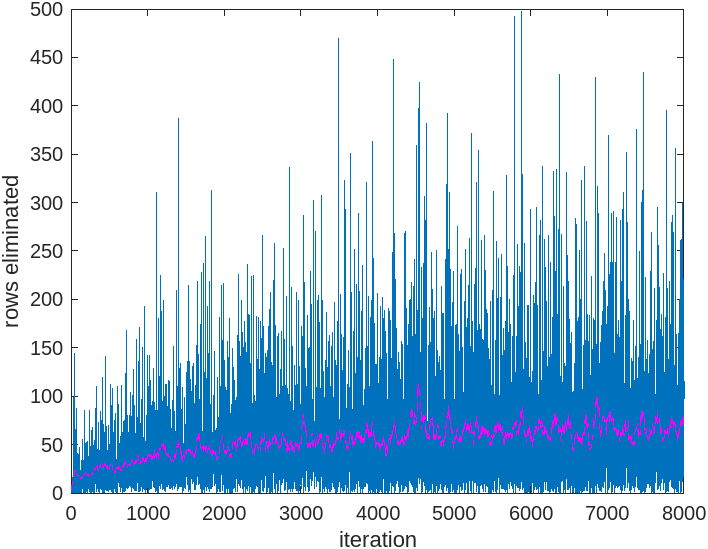
Below are the results of training an agent to play on an 8 x 8 board, with a batch size of one. The blue data points represent the result of each training iteration, while the magenta curve represents a moving average (window size: 50) of the scores. Following the magenta curve, it is evident that the algorithm is indeed learning.

Assessing Performance

We have already defined the score as the measure of performance, but how do we define good performance? It is reasonable to think of the quality of play by simply watching the agent play out the game. Hence the game board was reduced (from the standard 20 x 10 to 8 x 8 for this project) in order to more easily observe the agent losing. But this method of assessment is still fairly subjective; furthermore, it is comparitive, requiring multiple games to establish.

A more objective measure is by considering the number of pieces spawned w.r.t. the total number of rows cleared. Consider the case of an 8 x 8 board. In an ideal schenario, in which only the square puzzle blocks are played, it would take 4 of these puzzle pieces to clear 2 rows. The optimal ratio of spawned pieces to cleared rows for an 8-wide board is thus 2. This method of assessment also allows agents to be evaluated on single games as opposed to over many games.

Optimal play on an 8-wide board

In the demo'd case the final ratio at the end of the game is 2.038 (801 spawned pieces, 393 rows cleared). The resulting ratio is close to the ideal value but perhaps still has room for improvement. With more refined training methods and significantly more time spent on training, it may be possible to bring this value closer to the ideal value.

Out of curiosity I also tried the agent on a full sized 20 x 10 board, even though the agent has only been trained to play on an 8 x 8 board. In the case of a 10-wide board, we again imagine the case of only dropping square puzzle blocks. In this case, it would take 5 pieces to clear 2 rows — making the ideal ratio 2.5. The time for a game to play until completion was significant — a good sign for a quality agent. The agent successfully played through 100k pieces without the game terminating, clearing 3999 rows, resulting in a ratio of 2.5001. Excellent results! I am quite satisfied :).