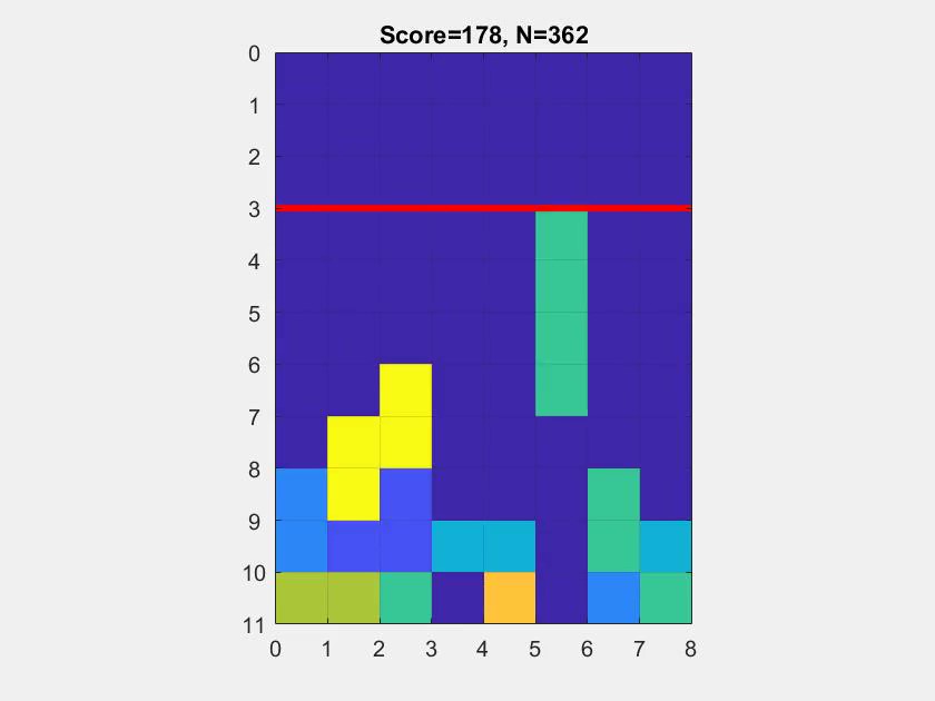
Figure 1; Video:

Intro

In this project, I use reinforcement learning to train an AI agent to play the game of Tetris. The agent is defined and trained with a custom set of cost functions in conjunction with vanilla policy gradient (VPG) training techniques.

The goal of an intelligent agent for Tetris is to clear as many rows as possible. For this project, the puzzle pieces are selected at random at each stage and the agent has no knowledge of the future sequence. The game plays until the puzzle stack overflows past the height limit (horizontal red line). The agent is strictly only allowed to drop a piece directly down into position. Note that variants of the game may have slightly different game rules.

Under the given game definitions, the problem of creating an intelligent agent is a NP-problem, meaning that we can only assess the performance of the agent after it has played a game. At first glance, one might try to optimize the agent by maximizing the number of rows cleared at each stage. However, through experiments, it quickly becomes clear that such a direct (‘greedy’) policy does not yield a very intelligent agent. Instead, we are able to achieve signficant improvements if we approach the problem with metaheuristics. These metrics are implemented through custom cost functions which are combined as a weighted sum to produce a policy (decision at each stage).

My primary interest in this project was to define these cost functions and to optimize their corresponding weights. The optimization strategy falls under the category of stochastic optimization, in which random perturbation is employed to adjust the weight (solution) vector.

Software & Simulation Tools Used

The system is modeled and simulated entirely within MATLAB computing environment.

Algorithm

Cost-to-go

We define the total cost of going from given state \(s_{k} \) (board configuration) to next state \(s_{k+1} \) as a linear combination of feature functions \(f \) with their corresponding weights. This cost can be written as:

where \(w_n \) denotes the weight corresponding to the \(n^{th} \) feature function \(f_{n} \) and \(N \) represents the total number of feature functions. Feature function \(f_{n} \) takes the current state \(s_{k} \) and an admissable control \(u_{k} \) as parameters and returns a real value. More compactly, this equation can be represented in vector form as:

At each stage, the goal of the agent is to choose an admissable control \(u_{k} \) such that the above expression is minimized. The optimal solution at stage \(k \) is thus,

Feature Functions

There are a total of 17 feature functions defined in this algorithm. The first, and most obvious one, is (1) score, which is defined as the number of rows cleared for a given admissable control. Other simple functions are (8) holes cost and (10) pile-height cost. Holes cost measures the number of occcupied cells with at least one cell above them and pile-height cost measures the height of the top most occupied cell.

Careful readers might notice that these feature functions more accurately represent a mix of cost and reward functions (as opposed to strictly a set of cost functions). Intuitively, an agent should maximize the result of (1) while minimizing the values of (8) and (10). Intuition tells us that we should incorporate these functions into Eqn. 1 by setting the sign on reward and cost functions oppsite to each other. In practice, as feature functions become more abstract, this relationship becomes less obvious, and the exact values of \(w_{n} \) (sign and magnitude) are entirely determined through training. The weights after training are often surprising, as they do not neccessarily follow intuition.

Training

The general structure of training is described below:

To begin training, I first give a seed value to \(\textbf{w} \). The values given are purely speculative but often give the system a head start in converging towards an optimized value.

In the first round of training, a batch of games are played with this seed value, and the average score (\(p\)) is recorded at the end of it. In the following training iteration, \(\textbf{w}\) is randomly ‘jiggled’ (randomly perturbed) and a batch of games are played using this perturbed vector \(\textbf{w}^{+}\). The average score of the new batch (\(p^{+}\)) is compared to the previous score. If the new score is higher (\(p < p^{+}\)), then the perturbed weights are allowed to become the new weights of the agent (\(\textbf{w} := \textbf{w}^{+} \)), and the direction of the perturbation (perturbation vector) is recorded. Otherwise, the perturbed weights are discarded and the original weights are preserved.

In the subsequent training iteration, the weights are perturbed either 1). in the direction of the perturbation vector (scaled by learning rate \(\alpha \) ) or 2). randomly jiggled again, depending on the outcome of the previous score. The process is repeated many times, until the values of \(\textbf{w} \) settle (converge) around a value.

We can make the training process slightly more sophisticated by imposing conditions on learning rate \(\alpha \) or the comparison condition (\( (p < p^{+})? \)). A classic approach is to define \(\alpha \) as an exponentially decaying value for each subsequent training iteration:

where \(\alpha_{0} \) is the initial learning rate, \(A\) is the decay rate, and \(t \) is the training batch number. We can see that as the training progresses, the perturbation on \(\textbf{w}\) becomes less and less, which in turn help the weights converge.

To reduce training noise, I have also found that by limiting how quickly \(p \) as a comparison point (threshold) changes, the learning progress tends to be more stable. Define:

Here, instead of letting \(p \) take on the value of \(p^{+} \) directly (\(p := p^{+}\)) when there is an improvement in performance, the threshold is instead increased by a value proportional to the difference between \(p\) and \(p^{+}\). The scaling factor \(\beta \) is set relatively small. The reason for this is because if an agent performs well during an iteration of training, we do not want to suddenly raise the bar for performance improvement — doing so would in some sense be punishing the agent for doing well.

Results

Below are the results of training an agent to play on an 8 x 8 board, with a batch size of one. The blue data points represent the result of each training iteration, while the magenta curve represents a moving average (window size: 50) of the scores. Following the magenta curve, it is evident that the algorithm is indeed learning.

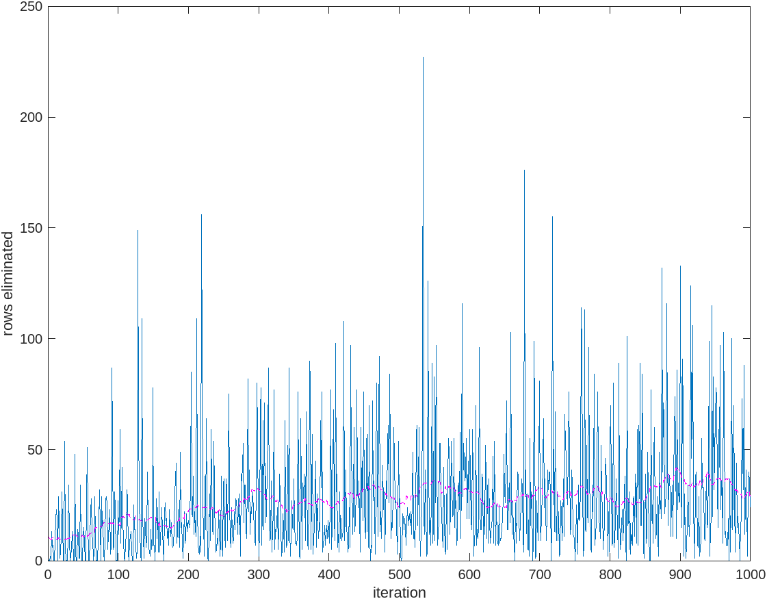
a) 1000 iterations

b) 8000 iterations

Figure 2: Score progression during training

Assessing Performance

One question that arises here is ‘how do we know if the algorithm is a good algorithm?’. We have already defined the score as the measure of performance, but how do we define ‘good’ performance? It is reasonable to think of the quality of play by simply watching the agent play out the game (hence, the reduced game board, to observe the agent losing), but this is still fairly subjective. A more objective measure is by considering the number of pieces spawned w.r.t. the total number of rows cleared. Consider the case of an 8 x 8 board. In an ideal schenario, in which only the square puzzle blocks are played, it would take 4 of these puzzle pieces to clear 2 rows; the optimal ratio of spawned pieces to cleared rows for an 8-wide board is thus 2.

In the demo case the final ratio at the end of the game is 2.038 (801 spawned pieces, 393 rows cleared). The resulting ratio is close to the ideal value but perhaps still has room for improvement. With more refined training methods and significantly more time spent on training, it may be possible to bring this value closer to the ideal value.

Out of curiosity I also tried the agent on a full sized 20 x 10 board, even though the agent has only been trained to optimize for an 8 x 8 board. In the case of a 10-wide board, we again imagine the case of only dropping square puzzle blocks. In this case, it would take 5 pieces to clear 2 rows — making the ideal ratio 2.5. The time for a game to play until completion was significant — a good sign for a quality agent. The agent played through 100k pieces without the game terminating, clearing 3999 rows, resulting in a ratio of 2.5001. Excellent results! I am quite satisfied :).