Figure 1

Intro

Planar compass-gait bipedal robots have been studied extensively in the dynamic walking community. Its kinematics are motivated by the the pendular efficiencies of human walking.

For this project, the robot is modeled as a purely passive system. Its movement relies solely on gravity and the resulting pendular motion of its legs. The robot is modeled through its equations of motion, derived using a combination of Newton-Euler and Lagrangian mechanics (TMT-method, presented by Vallery and Schwab). To model the robot’s interaction with the environment, the impact dynamics are simplified to maintain stability in simulation. The walker/robot is made to walk down a sloped surface, defined by road grade \(\gamma \). After simulation, the states of the system are plotted — from which we can observe the limit cycles, bifurcation, and eventually, chaos..

Software & Simulation Tools Used

The system is modeled and simulated entirely within MATLAB computing environment.

System Definitions

Below is a sketch of the system we are interested in. The walker interacts with the environment with its two rigid, rectangular legs. It is allowed to traverse along a sloped surface, defined by road grade \(\gamma \) through passive dynamics (gravity only, no other control inputs). At any given moment, one leg is denoted as the “stance leg” and the other as the “swing leg”. Corresponding states of the system are denoted by subscripts \(st \) & \(sw \), respectively.

Figure 2: sketch of cg-walker

Additionally, Each leg of the robot has a center of mass (CoM) located by an offset \(B \) and \(C \), and the ends of the legs are radiused (radius: \(R \)), allowing the walker to roll its ‘feet’ along the ground upon impact.

Finally, the states of the system are defined by the vector \([\phi_{st},\phi_{sw},\dot{\phi}_{st},\dot{\phi}_{sw}]\).

Impact Modeling

Contact and collision in the system is characterized by non-slip and no-bounce contact. Under such definition, translational momentum at the point of contact is not conserved. This simplification is reasonable for most low road grade simulations, where impact is relatively low. In this project, the system is necessarily operated at low road grades, because beyond a certain angle \(\gamma \), it is not possible to keep the walker from falling over. Furthermore, it allows us to reduce the number of states to simulate, as the position and translational velocities of the legs become coupled with the angle and angular velocities of the legs. As such, the system is completely described by the states \([\phi_{st},\phi_{sw},\dot{\phi}_{st},\dot{\phi}_{sw}]\).

Bifurcation

In order to observe bifurcation of the system, the walker should be maintained such that it does not fall over. If the robot were to fall over, its corresponding states likely do not belong to a limit-cycle we are interested in.

To aid in observing its limit cycles, the robot begins its simulated walk at an inital state close to one of its attractors. Doing so helps to 1). ensure that the walker does not fall over during simulation and 2). reduce the number of simulated steps required before periodic motion begins to emerge.

It typically takes some number of steps before the system begins to settle towards its attractors; and that to observe bifurcation, many more additional steps are required to observe their periodic orbits. According to Strogatz, a good starting value to begin observing bifurcation is on the order of a few hundred cycles (~300). In other words, producing a bifurcation diagram over some system variable (in this case, \(\gamma \)) quickly becomes a computationally heavy task, depending on the the level of granularity.

After simulating over about 10,000 increments of \(\gamma \) — 600 steps for each value of \(\gamma \) — it becomes evident that the states are indeed exhibiting bifurcation and chaotic behavior.

a) \(\phi_{st}\)

b) \(\phi_{sw}\)

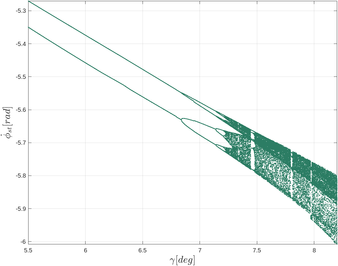
c) \(\dot{\phi}_{st}\)

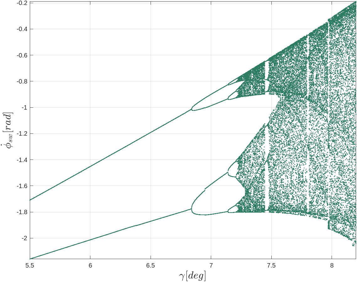
d) \(\dot{\phi}_{sw}\)

Figure 3: bifurcation diagram of system states

Using MATLAB’s plotting functions, we can iteratively plot the points along the robot w.r.t the simulated system states. The resulting animation serves as a visual sanity check, providing confidence that the system has been modeled as intended.

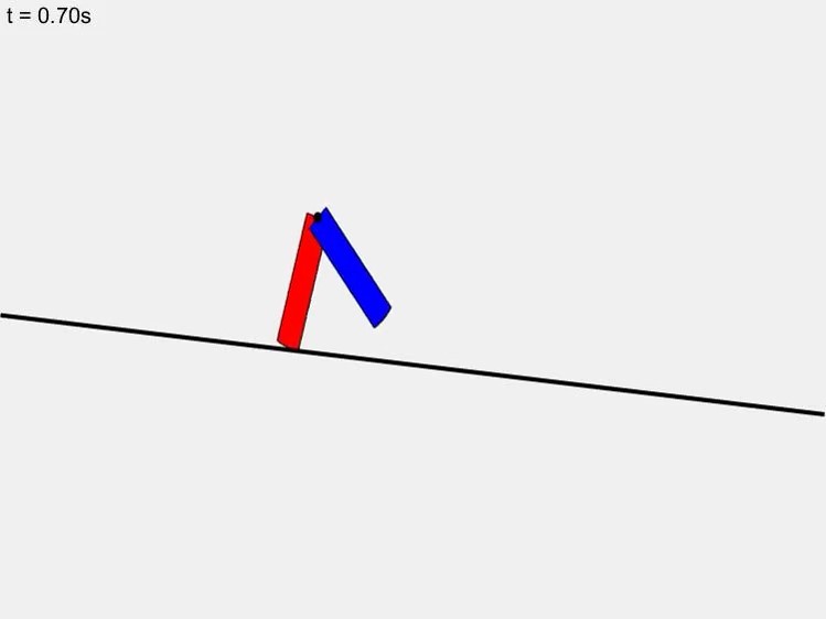
Video: animated motion using simulated states

References

Heike Vallery and Arend L. Schwab, “Advanced Dynamics”, 3rd edition, Delft University of Technology, 2020, ISBN/EAN 978-90-8309-060-3

Steven H. Strogatz, “Nonlinear Dynamics and Chaos: With Applications in Physics, Biology, Chemistry, and Engineering”, Addison-Wesley Pub., 2000, ISBN 9780201543445